# (a) What time does the ball hits the ground with t_intervals = 0 - 5
# Basic numPy
import numpy as numpy
h0 = 100 # initial hight, in m
g = 9.81 #gravization in m/s^2
# Creating numpy arrays (np.linspace(start, stop, num) => the range built-in
t = np.linspace(0, 5, 50) # time interval
# Position as a function of time
y = h0 - 0.5 * g * t**2
# time the ball hits the ground
t_ground = np.sqrt(2*h0/g)
print('(a) Ball hits the ground at t=',round(t_ground, 3), 's')
# Calculate the initial velocity of the ball
v_ground = g * t_ground
print('(b) velocity at the ground =',round(v_ground, 3), 'm/s')
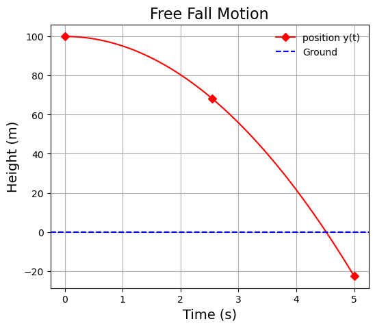
# Set plot the position of the ball vs time as it falls.
import matplotlib.pyplot as plt
plt.figure(figsize=(6,5))
plt.plot(t, y, marker='D', markevery=[0, 25, -1], color='r', label='position y(t)')
plt.axhline(0, color='blue', linestyle='--', label='Ground')
plt.title('Free Fall Motion', fontsize=16, fontname='Sans serif')
plt.xlabel('Time (s)', fontsize=14, fontname='Sans serif')
plt.ylabel('Height (m)', fontsize=14, fontname='Sans serif')
plt.legend()
plt.legend(framealpha=0)
plt.grid(True)
plt.show()
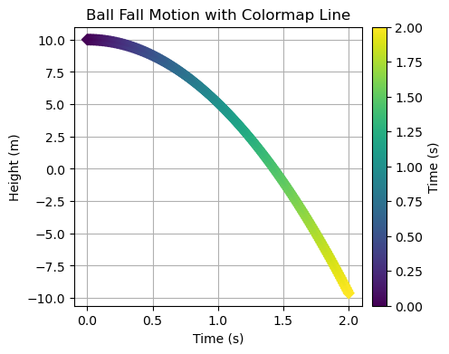
# Scatter plot with color map
import numpy as np
import matplotlib.pyplot as plt
from matplotlib.collections import LineCollection
t = np.linspace(0, 5, 50)
y = h0 - 0.5 * g * t**2
# Create segments for line
points = np.array([t,y]).T.reshape(-1, 1, 2)
segments = np.concatenate([points[:-1], points[1:]], axis =1)
# colormap
Lc=LineCollection(segments, cmap='plasma', linewidth=3, norm=plt.Normalize(t.min(), t.max()))
Lc.set_array(t) # color by time
fig, ax = plt.subplots(figsize=(5,4))
ax.scatter(t, y, c=t, cmap='plasma', marker='D')
ax.add_collection(Lc)
ax.autoscale()
# Adding colorbar
cbar = plt.colorbar(Lc, ax=ax, pad =0.02)
cbar.set_label('Time (s)')
ax.set_xlabel('Time (s)')
ax.set_ylabel('Height (m)')
ax.set_title('Free Fall Motion')
plt.grid(True)
ax.set_axisbelow(True)
plt.savefig('Fallmotion_colormap.svg', bbox_inches='tight')
plt.show('Free Fall Motion')